


Both languages are highly popular in data science and machine learning. Python is an easy to learn general purpose language, while R was developed mainly for statisticians. Although there is a large amount of overlap between the languages, people with a background in statistics seem to prefer R over Python. On the other hand people new to programming or without a sufficient background in statistics prefer Python because of it's easy to learn syntax.
Personally I think it is more a matter of choosing the right tool for the job. I would use Python for creating complex deep learning models and use R to analyze the results afterwards. In this blog I will show you that it is actually possible to do both using R on SQL server.
I will use an actual project done by Thinkwise as an example. Several years ago Nedstaal asked Thinkwise to replace an outdated tool that was capable of predicting the hardenability of steel given it's chemical composition using a neural network. With the more limited possibilities back then it was decided that the best we could do was to create a web service and communicate with it through custom GUI tasks.
In this blog I will demonstrate that there is no need for such a complicated setup anymore and that every step that is necessary to create, train and use neural network can now be directly integrated in SQL templates.
For this blog I will demonstrate how to integrate R in your projects.
Deep learning frameworks
Most deep learning frameworks are developed either for Python or R. Some, like Keras and Tensorflow, actually have implementations for both. In this blog I will use the R implementation of Keras, which is not a deep-learning framework in itself, but actually a high-level api on top of several other actual deep learning frameworks. At the moment Tensorflow, Theano and Microsoft Cognitive toolkit are supported. For quickly setting up deep learning models, like the multi-layered perceptron (MLP) we will be using in this blog, Keras helps by automating many steps you would otherwise have to program yourself in one of the mentioned frameworks.
Google did however acknowledge the usefulness of a simplified API and has now made it part of their Tensorflow distribution. Meaning that in Tensorflow you can now quickly setup a network using Keras and directly use all the advanced functionality that Tensorflow offers. In the upcoming 2.0 version of Tensorflow, they will completely merge it with Keras. At present you can build models using both Tensorflow or Keras functions, in the future all the overlapping functions will be removed and replaced by Keras functions.
As mentioned I will now be only using one of the most simple types of neural networks, the MLP, but before going on with my story on Nedstaal I want to give you some other examples of what such deep learning frameworks are capable of. One very common application is recognizing objects or faces in images or even movies.
Currently the area of machine learning that receives the most attention is Reinforcement Learning. You probably all heard of AI reaching superhuman performance on ATARI games or beating the world champion in GO. More recently AI's performance in DOTA 2 and Startcraft reached the news.
But there is so much more what you can do with such frameworks. For instance this example of how a neural network is used to create a text-to-speech system which sounds almost perfectly human.
Another type of application I personally find very impressive are generative adversarial networks or GAN for short. See this post on medium.com for some cool examples of what such networks are capable of.
After reading all the impressive applications of AI, creating a simple MLP to predict the hardenability of steel may sound a bit underwhelming by now. However keep in mind that we are building it using a framework in which you are able to actually create all the examples mentioned above. The Tensorflow version called using Microsoft Machine Learning Services is exactly the same Tensorflow as you would use in a normal Python or R project.
Nedstaal

Nedstaal was a company that produced steel. Unfortunately they went bankrupt a few years ago and now the only steel producing company left in The Netherlands is Corus.
Steel in fact is produced from iron ore and scrap. This can contain impurities which can impact the quality of the steel. On top of that certain alloying elements can be added to produce different grades of steel. Together the concentrations of elements present thus determine the quality. A standard way of describing steel is actually by mentioning the concentrations of important alloys. For instance 1% Cr, 0.25% Mo and 0.4% C
One of the factors that is influenced by the presence of those chemicals is hardenability. Normally for each quality of steel a hardenability profile can be acquired by performing a standardized test called the Jominy End Quench Test. During this test the hardness profile will be determined by measuring the hardness, expressed in HRC at different distances. See https://en.wikipedia.org/wiki/Hardenability for more information on this subject.
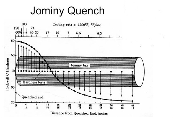
A big disadvantage of this test is that it is time-consuming and very expensive. Luckily research actually done at Nedstaal showed that it is actually possible to predict these HRC values with a pretty high degree of accuracy using a Neural Network, given the concentrations of various elements present in that steel quality. You can find the original paper here
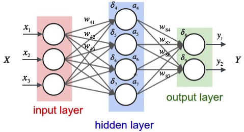
The type of neural network they used is called a multilayer perceptron, or MLP for short, and typically consists of three layers.
- The input, in our case the different concentrations of the elements;
- A hidden layer;
- The output layer, returning the HRC values at different distances.
As mentioned in the introduction Thinkwise was asked to replace their outdated tool, and in this blog I will show how you can now easily build such an application with the help of Microsoft Machine Learning Services.
Setting up your environment
Before we can do anything I have promised above, a necessary first step is to make sure everything is setup properly. Unfortunately there are quite a few steps required, but on the positive side you only have to do this once.
Preparing SQL Server
The first thing we need to setup correctly is SQL server. You will need at least SQL Server 2017 and enable R and Python during installation. Microsoft has a good tutorial here.
Unfortunately the standard installation of SQL server 2017 ships with a very outdated R distribution. Most of the R packages I will be using in this blog post are not compatible with such an old version, thus it is important to get a more recent one. Luckily Microsoft is aware of that and gives us a method to get a recent enough R distribution by upgrading Machine Learning Service (MLS), look here for more information.
Setting up R
When SQL server is set-up correctly you will find a R distribution in the C:\Program Files\Microsoft\ML Server\R_SERVER folder. The same is true for Python for which Microsoft installs an Anaconda distribution. This can be found in the PYTHON_SERVER folder.
This R distribution that is used by SQL server when executing R scripts from SQL is, besides some modifications done by Microsoft, a complete R distribution. Although the R distribution that ships with MLS 9.3 has a comprehensive list of installed packages, we do need to install a few additional additional packages for everything to work. We thus need a method to install those packages in such a way that R scripts executed from SQL can use them. The easiest way to do this is by installing Rstudio on the SQL Server machine.
R packages
Besides the standard packages offered by R, we will need the following packages and their dependencies installed in the system library.
- devtools
- tidyverse
- keras (tensorflow)
Devtools
In almost all cases packages are published on CRAN and installing new packages can be done easily by simply executing in a RStudio console:
code:
Or use the package installation function provided by Rstudio.install.packages("devtools")However, some packages are not available on CRAN or the versions published there are too outdated. In that case you must build and install the packages from source code. This does require you to have Rtools installed on your system. R packages can be written in different languages besides R, like C or FORTRAN and Rtools provides compilers and other necessary tools to build such packages.
The main reason I am mentioning this is that we will need Keras and Tensorflow and both packages are not on CRAN. They are only available as source code on github, which is also true for some of it's dependencies.
Please don't be scared off now, because devtools actually makes this procedure pretty easy. It has several functions to install from code repositories, including github. One of such packages that needs to be installed this way is Keras and this can be done by executing the following line of code in a RStudio console.
code:
devtools::install_github("rstudio/keras")
This will first pull all source code from github. After that it will run the appropriate compiler, build the package, do some integrity checks and if all went well install it.
Tidyverse
The tidyverse library is actually a collection of different R packages designed for data science.
I highly recommend looking at the cheat sheets available at https://www.rstudio.com/resources/cheatsheets/ to see what these packages are capable of.
Throughout this blog post almost all data manipulation and visualization is done using one or more tidyverse packages. Especially the dplyr package is used extensively, because this gives us an easy to use but very powerful syntax for data manipulation. In my opinion far superior to T-SQL.
This package is available on CRAN and can be installed in the same way as devtools.
Keras / TensorFlow
Although we will only create a simple neural network in this blog and there are standard packages available in R to do that, I take the opportunity to showcase that with Machine Learning Services it is now possible to use complex deep learning frameworks directly from T-SQL.
I chose Keras which in itself is not a deep learning framework, but offers a high level API to access several deep learning frameworks, like Tensorflow, Theano or Microsoft Cognitive toolkit.
Keras simplifies creating and using deep learning models in these different frameworks. For more complex situations I would use Tensorflow directly, but for the relatively simple model used in this blog Keras is the perfect tool for the job.
Since Keras works on top of other frameworks it is necessary to have at least on of them installed on the system. Keras is standard configured to use Tensorflow and since this is also my personal favorite, I recommend installing that.
Both Keras and Tensorflow have R implementations, but rely on their original python distributions. Look here for more information. The tutorial mentions installing the python version of Keras and Tensorflow by using the install function from the R packages, but for me it worked best to directly install Keras and Tensorflow in the python distribution that came with MLS using pip.
Building the application
I want to emphasize that the main focus of this blog post is to demonstrate how you can integrate R functionality in T-SQL scripts and less on actual R programming. I will thus not demonstrate everything that is necessary for data preparation, building and training the model etcetera. Instead I created a package called called ThinkwiseMLP which already contains all of this. This package exposes the two functions needed for our purpose, namely training new models and using trained models to predict HRC values.
In a follow-up blog, I will go into much more detail everything about everything that was necessary to create this ThinkwiseMLP package.
This method of first creating a package before using the R integration in SQL server is also the preferred workflow. This way you can keep the lines of R code necessary in your SQL templates to a minimum. The SQL Server Management Studio does not provide you with any R debugging tools or even syntax highlighting. Doing most development in a R IDE is thus highly recommended.
Training the neural network
Since the type of neural network that is used here will be trained using a so-called supervised method we will need both the chemical concentrations and measured HRC values at different distances. Data for training is stored in two tables. One called dataset and contains rows with an id and a description for a dataset. The other one, dataset_rows contains the actual data and has the id from the dataset table as it's foreign key. A simple setup to create and use multiple datasets. You will want multiple datasets, because creating the perfect dataset to train the network can be quite an art.
This is very much true for Nedstaal. They provided us with two datasets. One with at least 5000 older measurements and some 500 newer measurements. There is a time gap of a least ten years between the measurements in both sets. This doesn't have to be problematic, but for Nedstaal it was. The qualities of steel Nedstaal produced has changed over time and the older dataset is pretty outdated. Tests show that a network trained on the old data does a very bad job on predicting the new data and vice versa. We thus need a good balanced set of old and new data.
There is another problem with the data and that is that the older dataset has a lot of missing values. Measurements with HRC values lower than 20 were seen as unreliable and are recorded as zeros in the dataset. This is a real problem that has to be solved, but for the purpose of this blog I will use an already prepared dataset.
Code template training task
Before diving into the code, I like to mention that I actualy created a working demo application and the code I am showing here is from the actual SQL task templates. The only adjustments I made for this blog is defining some variables which in reality were task input variables.
code:
declare @epochs int = 1000
declare @hidden_units int = 50

-- Select the training data
declare @query nvarchar(max) = 'select * from dataset_rows where set_id = '+cast(@set_id as varchar)

-- Define the output variables
declare @fitted_model varbinary(max)
declare @train_plot varbinary(max)
declare @train_mse float
declare @val_mse float

EXEC sp_execute_external_script
@language = N'R'
, @script = N'
# Specify python location for Keras/Tensorflow
require(tidyverse)
tensorflow::use_python("C:\\Program Files\\Microsoft\\ML Server\\PYTHON_SERVER\\python.exe")

# Prepare and split data
data<-data %>% rename(id=row_id) %>% select(-set_id)
input <- data %>% select(-starts_with("J"))
output <- data %>% select("id", starts_with("J"))

# Fit the model
train_results <- ThinkwiseMLP::trainNeuralNetwork(input, output, epochs=epochs, h=hidden)

# Serialize to the fitted model
# So it can be saved to the database
fitted_model <- serialize(train_results$fitted, connection=NULL)

#Create a plot of the training progress
image_file = tempfile()
#Create png graphics device
svg(filename = image_file)
#For some reason print is necessary in some cases
print(plot(train_results$history, smooth=FALSE))
dev.off()

# serialize image
train_plot <- readBin(file(image_file,"rb"),what=raw(),n=1e6)

#Train and validation MSE
train_mse <-train_results$history$metrics$loss %>% last
val_mse <-train_results$history$metrics$val_loss %>% last
'
,@input_data_1 = @query
,@input_data_1_name= N'data'
,@params = N'@epochs int
            ,@hidden int
            ,@fitted_model varbinary(max) OUTPUT
            ,@train_plot varbinary(max) OUTPUT
            ,@train_mse float OUTPUT
            ,@val_mse float OUTPUT'
,@epochs = @epochs
,@hidden = @hidden_units
,@fitted_model = @fitted_model OUTPUT
,@train_plot = @train_plot OUTPUT
,@train_mse = @train_mse OUTPUT
,@val_mse = @val_mse OUTPUT
R code is always executed by calling the sp_execute_external_script procedure. Important to know is that if you need data from a table or view you need to pass a query to the @input_data_1 parameter. As you can see I declared the @query variable for that purpose. The result of that query will become available in R as a dataframe variable. The @input_data_1_name parameter will determine the name of that dataframe in R. In this case I just called it data.
Besides tabular data it is also possible to pass on scalar variables. The @params variable expects a string containing all variables and their datatypes separated by a comma. What I found a little confusing at first is that the variables in this list are actually the names used in R except the leading @ character.
What follows are the actual mappings of the names used in R and the SQL variables. Thus the line @hidden = @hidden_units means that the variable is called hidden in R and is mapped to the SQL variable @hidden_units. Variables flagged with OUTPUT will receive the values of their mapped R variables after the stored procedure has finished.
As you can see in this example we have two variables which only act as input to the R script, @epochs and @hidden_units. In the actual application these variables are task input variables, so a user can provide them in the task pop-up. The @set_id variable can have a reference to the dataset table, so that the train task can be executed on a specific dataset.
Training the network
The R code itself is hopefully pretty self-explanatory, but a few things are useful to mention. The data that is put in the data object by the select query contains both the input and output data and a column set_id we do not need.
Before training it is important that we split the data in an input dataframe containing the chemical concentrations and an output dataframe containing the measurements in HRC values. In this specific example all measurement columns start with a "J", which we can use to our advantage in splitting.
Training itself is initiated by calling the trainNeuralNetwork from the ThinkwiseMLP package.
code:
# Prepare and split data
#Renaming row_id to id because the code library is build to use id as columnname
data<-data %>% rename(id=row_id) %>% select(-set_id)
input <- data %>% select(-starts_with("J"))
output <- data %>% select("id", starts_with("J"))

# Fit the model
train_results <- ThinkwiseMLP::trainNeuralNetwork(input, output, epochs=epochs, h=hidden)
The train_results object that is given back by the function is actually a structure containing both the trained model and an object that has some statistics about the training progress.
code:
# Trained model
train_results$fitted
# Training statistics
train_results$history
Saving a trained model
At this point training is finished and all the remaining R code is only there to send back some useful data. The most important one is the actual trained model. We do not want to train a model every time before we want to do a prediction, thus saving the model so it can be reused on a later time is a must. Luckily this is easy enough. We already defined the SQL variable @fitted_model of type varbinary(max) and added it to the list of variables in the sp_execute_external_script procedure and flagged it as OUTPUT.
The only thing you now need to do is to serialize the trained_model and save it as fitted_model.
code:
fitted_model <- serialize(train_results$fitted, connection=NULL)
When the stored procedure code is finished, the @fitted_model variable will now contain binary data that can be stored in the database. If at some later point in time we want to use that same model, the only thing we need to do is to map it as a varbinary(max) variable to the sp_execute_external_script procedure stored procedure and in R code call deserialize to restore it back to its original object.
Returning useful training statistics
Having a stored model is nice, but actually pretty useless is we have no idea about how well it performs. Not only is it useful to know the performance of the model you just trained, but since you probably will be training many models using different configurations and on multiple data sets, you should have ways of comparing them. Of course you could do some testing afterwards, but since the trainNeuralNetwork function already provides us with such information it would be stupid not using that.
I think plots give the most useful information about the quality of trained model, so I decided that I want the stored procedure to return that as well. The train function will actually internally split the data in two sets. One that is used for training and one that is used to test the network on data it was not trained on. In the ideal situation performance on both sets should be identical.
How good a network is in predicting is expressed by a loss function called the Mean-Squared Error (MSE). I will not go into much detail about how this value is determined, for now it is sufficient to know that lower is better.
During an optimal behaving training process this value should decrease over time for both the training and validation data. Thus what I actually want to see in the plot is exactly that. Since R is developed mainly for statisticians, they knew people would be interested in such a plot, thus creating it is very easy. By just calling the plot function on the train_results_history object it will give us exactly what we want.
However the plot is now only available in the R context and we will need to perform a few tricks to get it back in SQL. To do this you need to tell R that the actual plot needs to be printed on an image, in this case of type SVG, and serialize the actual image back to the variable train_plot. Similar to returning the model, the plot will now be stored in the @train_plot SQL variable.
code:
#Create a plot of the training progress
image_file = tempfile()
#Create svg graphics device
svg(filename = image_file)

#For some reason print is necessary in some cases
print(plot(train_results$history, smooth=FALSE))

# Change graphic device back to default
dev.off()

# serialize image
train_plot <- readBin(file(image_file,"rb"),what=raw(),n=1e6)
I return the final train_mse and val_mse as well. Since they are useful for a quick comparison between the trained models.
code:
#Train and validation MSE
train_mse <-train_results$history$metrics$loss %>% last
val_mse <-train_results$history$metrics$val_loss %>% last
Using the model to do predictions
For predicting we need the trained model and concentrations of the chemical elements as input. In the demo application we have a table called Steel that contains different qualities and it is assumed that a previously trained model is saved in the table fitted_models in the column model. What is nice about all the values we returned after the training is that they are now very useful for selecting the best model for predicting, as you can see in the next task parameter popup.
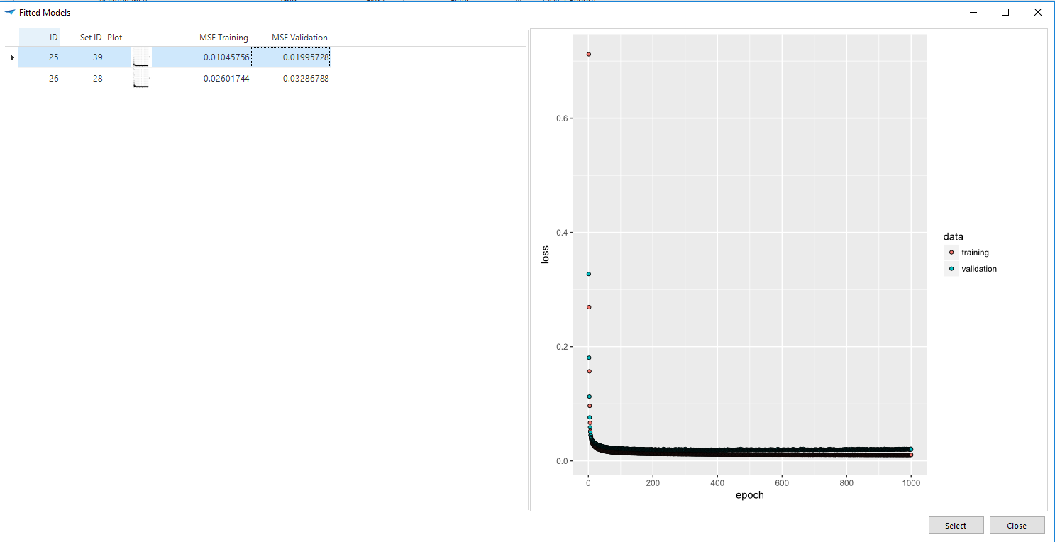
When comparing MSE values, the validation MSE is the most important. Model with id 25 has the lowest values, so I select that one.
The next piece of code shows how we can load the saved model with id 25 and do a prediction on all rows in the steel table.
code:
declare @model_id int = 25
declare @model varbinary(max) = (select model from fitted_models where model_id = @model_id)

create table #result ( steel_id int
                      ,distance varchar(4)
                      ,hrc numeric(5,2)
)

declare @input nvarchar(max) = 'select steel_id as id, C,Mn,Si,Cr,Ni,Mo,B,Al,N from steel'

insert into #result
EXEC sp_execute_external_script
@language = N'R'
, @script = N'
#Predict HRC values.
# Point R to the python distribution that contains Keras/Tensorflow
tensorflow::use_python("C:\\Program Files\\Microsoft\\ML Server\\PYTHON_SERVER\\python.exe")
model <- unserialize(fitted)
result <- ThinkwiseMLP::predictHRC(model, data)
'
, @input_data_1 = @input
, @input_data_1_name= N'data'
, @output_data_1_name = N'result'
, @params = N'@fitted varbinary(max)'
, @fitted = @model
I already explained most of how to use the sp_execute_external_script in the previous section, but there is one thing that is different in this case that needs to be mentioned. In the previous example all data was returned using output variables. In this case one row of input data will give back 15 rows of measurement predictions and we are not restricted in using just one row of input data. Thus we need tabular output instead of scalars now.
For the procedure to return a table, we need to specify which R dataframe needs to be returned. By giving the variable @output_data_1_name a value, "result" in this case, the stored procedure knows that the contents of that dataframe has to be returned. A restriction here is that only objects that are of class "data.frame" can be returned this way.
What is nice to see here is that the previously stored neural network is loaded from the fitted_models table, selected in the @model variable which is then mapped to the variable fitted in R. The only thing we need to do before we can actually use the model is unserialize so it changes back to it's original R format. After that we pass the model and the input data to the predictHRC function and the result object will contain all the predictions.
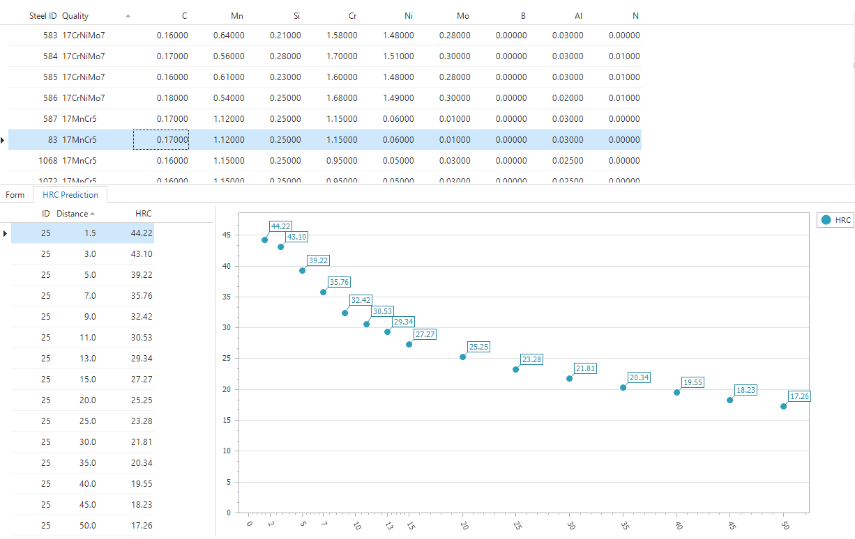
Since it is not possible to directly query the results from a stored procedure, you need to store it in some table structure before you can do something with the results. In this case I insert the results in the temp table #results. What you may have noticed is that this table only has three columns, meaning that the data is actually transformed from wide format, each measurement in a different column, to long format where all measurements are in one columns. Long format is necessary when you want to plot your results, for instance by using our own cube component.
Concluding Remarks
What we have achieved in what I think are just a few lines of not too complicated code is training a neural network using an advanced deep learning framework. Have a method to return the trained model so it can be used later on and return both a graph and numerical values useful for analyzing and comparing the performance of trained models. Furthermore we have a method to load a previously trained network and use it to predict hardenability.
Best of all, by integrating R (or Python) to SQL templates in Thinkwise projects this opens the door to a whole new wealth of possibilities.